Shared Memory

The asynchronous scheduler requires an apply_async function and a Queue. These determine the kind of worker and parallelism that we exploit. apply_async functions can be found in the following places

• multithreading.Pool().apply_async - uses multiple processes
• multithreading.pool.ThreadPool().apply_async - uses multiple threads
• dask.async.apply_sync - uses only the main thread (useful for debugging)

Full dask get functions exist in each of dask.threaded.get, dask.multiprocessing.get and dask.async.get_sync respectively.

Policy

The asynchronous scheduler maintains indexed data structures showing which tasks depend on which data, what data is available, what data is waiting on what tasks to complete before it can be released, and what tasks are currently running. It can update these in constant time relative to the number of total and available tasks. These indexed structures make the dask async scheduler scalable to very many tasks on a single machine.

To keep the memory footprint small we choose to keep ready-to-run tasks in a LIFO stack such that the most recently made available tasks get priority. This encourages chains of related tasks to complete before starting new chains. This is also queryable in constant time. Read more about our scheduling policy

Performance

tl;dr The threaded scheduler overhead behaves roughly as follows:

• 1ms overhead per task
• 100ms startup time (if you want to make a new ThreadPool each time)
• Constant scaling with number of tasks
• Linear scaling with number of dependencies per task

Schedulers introduce overhead. This overhead effectively limits the granularity of our parallelism. Below we measure overhead of the async scheduler with different apply functions (threaded, sync, multiprocessing), and under different kinds of load (embarrassingly parallel, dense communication).

The quickest/simplest test we can do it to use IPython’s timeit magic.

In [1]: import dask.array as da

In [2]: x = da.ones(1000, chunks=(2,)).sum()

In [3]: len(x.dask)
Out[3]: 1001

In [4]: %timeit x.compute()
1 loops, best of 3: 550 ms per loop

Around 500 microseconds per task. About 100ms of this is from overhead

In [6]: x = da.ones(1000, chunks=(1000,)).sum()
In [7]: %timeit x.compute()
10 loops, best of 3: 103 ms per loop

Most of this overhead is from spinning up a ThreadPool each time. This can be mediated by using a global or contextual pool

>>> from multiprocessing.pool import ThreadPool
>>> pool = ThreadPool()
>>> da.set_options(pool=pool)  # set global threadpool

or

>>> with set_options(pool=pool)  # use threadpool throughout with block
...     ...

We now measure scaling the number of tasks and scaling the density of the graph.

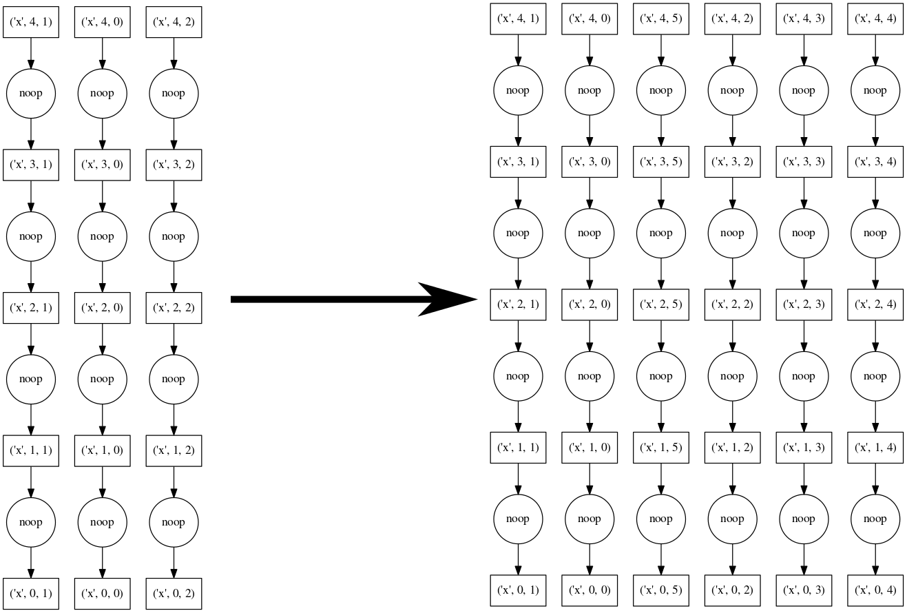
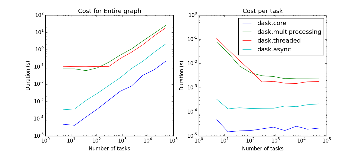
Linear scaling with number of tasks

As we increase the number of tasks in a graph we see that the scheduling overhead grows linearly. The asymptotic cost per task depends on the scheduler. The schedulers that depend on some sort of asynchronous pool have costs in the few milliseconds. The schedulers that are single threaded are down in the microsecond range.

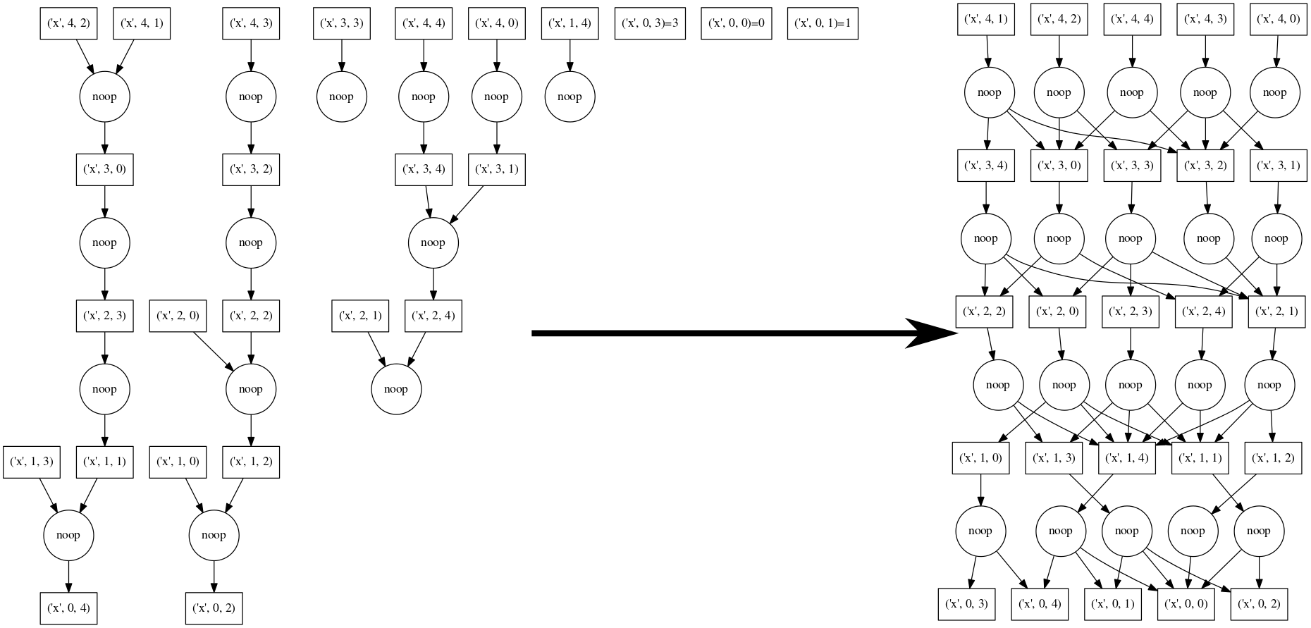
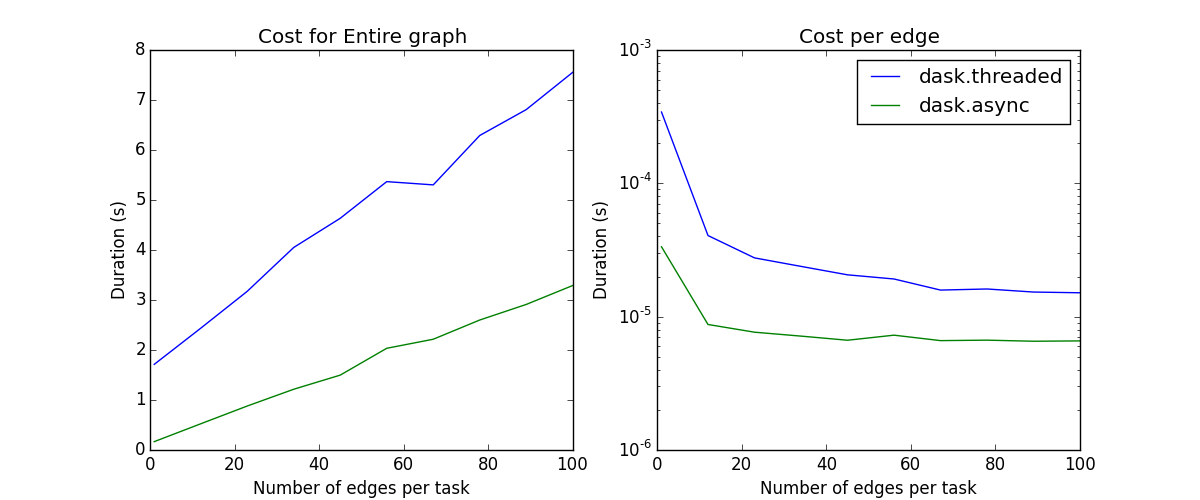
Linear scaling with number of edges

As we increase the number of edges per task we see that scheduling overhead again increases linearly. Note that neither the naive core scheduler nor the multiprocessing scheduler are good at workflows with non-trivial cross-task communication; they have been removed from the plot.

Script available here

Known Limitations

The shared memory scheduler has notable limitations:

1. It works on a single machine
2. The threaded scheduler is limited by the GIL on Python code and so, if your operations are pure python functions you should not expect a multi-core speedup.
3. The multiprocessing scheduler must serialize functions between workers; this can fail
4. The multiprocessing scheduler must serialize data between workers and the central process; this can be expensive
5. The multiprocessing scheduler can not transfer data directly between worker processes; all data routes through the master process